Autoencoder

An autoencoder is a neural network trained to copy its input to its output through a compressed bottleneck. The encoder maps the input into a lower-dimensional latent space, and the decoder reconstructs the original input from that latent representation.

In this notebook, we train an autoencoder on MNIST, visualize how the reconstructions improve throughout training, and plot the loss landscape of the encoder and decoder layers — following the same visualization style as the Neural Network notebooks.

Importing the libraries

import random
import numpy as np
import io

# %matplotlib ipympl
import matplotlib
matplotlib.use("Agg")
import matplotlib.pyplot as plt
from matplotlib.lines import Line2D
from mpl_toolkits.mplot3d import Axes3D
from PIL import Image as PILImage

from celluloid import Camera
import scienceplots
from IPython.display import Image

random.seed(0)
np.random.seed(0)
plt.style.use(["science", "no-latex"])

We will use the MNIST dataset. Each image is \(28 \times 28\) pixels, flattened into a \(784\)-dimensional vector before passing through the autoencoder.

We use all 60,000 images for training. A held-out split of 10,000 images supplies the 8 reconstruction and 16 loss-landscape visualization samples.

import torch
import torch.nn as nn
import torchvision
import torchvision.transforms as transforms
from torchvision.datasets import MNIST
from torch.utils.data import random_split, DataLoader, ConcatDataset

torch.manual_seed(0)
if torch.cuda.is_available():
    torch.cuda.manual_seed_all(0)
torch.backends.cudnn.deterministic = True
torch.backends.cudnn.benchmark = False

mnist_dataset = MNIST(
    root="data/", download=True, train=True, transform=transforms.ToTensor()
)

image_tensor, label = mnist_dataset[0]
print(image_tensor.shape, label)
print(torch.max(image_tensor), torch.min(image_tensor))
plt.imshow(image_tensor[0], cmap="gray")
plt.title(f"Label: {label}")
plt.axis("off")
plt.show()

torch.Size([1, 28, 28]) 5
tensor(1.) tensor(0.)

split_generator = torch.Generator().manual_seed(0)
train_data, validation_data, _ = random_split(
    mnist_dataset, [50000, 10000, 0], generator=split_generator
)
train_data = ConcatDataset([train_data, validation_data])

batch_size = 256
loader_generator = torch.Generator().manual_seed(0)
train_loader = DataLoader(
    train_data, batch_size, shuffle=True, generator=loader_generator
)

fixed_images = torch.stack([validation_data[i][0] for i in range(8)])

latent_count = 2000
latent_images = torch.stack([validation_data[i][0] for i in range(latent_count)])
latent_labels = torch.tensor([validation_data[i][1] for i in range(latent_count)])

Autoencoder

An autoencoder has two parts:

1. Encoder — compresses \(x \in \mathbb{R}^{784}\) into \(z \in \mathbb{R}^{2}\)

2. Decoder — reconstructs \(\hat{x} \in \mathbb{R}^{784}\) from \(z\)

The network minimizes MSE between \(x\) and \(\hat{x}\).

Encoder

\( \begin{align*} h_1 &= \text{ReLU}(W_1 x + b_1) \\ h_2 &= \text{ReLU}(W_2 h_1 + b_2) \\ h_3 &= \text{ReLU}(W_3 h_2 + b_3) \\ z &= W_4 h_3 + b_4 \end{align*} \)

Maps \(784 \rightarrow 512 \rightarrow 256 \rightarrow 64 \rightarrow 2\).

Decoder

\( \begin{align*} h_4 &= \text{ReLU}(W_5 z + b_5) \\ h_5 &= \text{ReLU}(W_6 h_4 + b_6) \\ h_6 &= \text{ReLU}(W_7 h_5 + b_7) \\ \hat{x} &= \sigma(W_8 h_6 + b_8) \end{align*} \)

Maps \(2 \rightarrow 64 \rightarrow 256 \rightarrow 512 \rightarrow 784\). The first decoder layer \(\text{Linear}(2, 64)\) has exactly 2 input weights per neuron.

Loss Function

\( \begin{align*} \text{MSE} = \frac{1}{n} \sum_{i=1}^{n} (x_i - \hat{x}_i)^2 \end{align*} \)

The target is the input itself — not the digit label.

Graphing functions

The graphing functions produce two animations:

• create_reconstruction_plots — MSE curve with original and reconstructed digits

• create_latent_plots — a large 2D scatter of the latent space on the left, with the MSE curve (top-right) and reconstructions (bottom-right)

• plot_latent_frame — projects the validation images to the 2-neuron bottleneck \(z\) and scatters them, colored by their true digit, so same-digit clusters emerge over training

• show_epoch — controls animation frame capture frequency

# Fixed color per digit so repeated runs always render identical GIFs.
DIGIT_COLORS = plt.get_cmap("tab10").colors


def create_reconstruction_plots(mse_ylim=(0, 0.08)):
    fig = plt.figure(figsize=(16 / 9.0 * 4, 4 * 1.2), layout="constrained")
    fig.suptitle("Autoencoder Reconstructions")

    gs = fig.add_gridspec(2, 2, width_ratios=[1, 1])
    mse_ax = fig.add_subplot(gs[:, 0])
    orig_ax = fig.add_subplot(gs[0, 1])
    recon_ax = fig.add_subplot(gs[1, 1])

    mse_ax.set_xlabel("Epoch", fontweight="normal")
    mse_ax.set_ylabel("Error", fontweight="normal")
    mse_ax.set_title("Mean Squared Error")
    mse_ax.set_ylim(mse_ylim)

    orig_ax.axis("off")
    orig_ax.set_title("Original")
    recon_ax.axis("off")
    recon_ax.set_title("Reconstructed")

    camera = Camera(fig)
    return mse_ax, orig_ax, recon_ax, camera


def create_latent_plots(mse_ylim=(0, 0.08), epochs=None):
    fig = plt.figure(figsize=(16 / 9.0 * 4, 5), layout="constrained")
    fig.suptitle("Autoencoder Latent Space")

    gs = fig.add_gridspec(2, 2)

    latent_ax = fig.add_subplot(gs[:, 0])
    latent_ax.set_title("Latent Space $z$ (colored by digit)")
    latent_ax.set_xlabel("$z_1$", fontweight="normal")
    latent_ax.set_ylabel("$z_2$", fontweight="normal")
    latent_ax.set_xlim(-25, 25)
    latent_ax.set_ylim(-50, 50)

    mse_ax = fig.add_subplot(gs[0, 1])
    mse_ax.set_xlabel("Epoch", fontweight="normal")
    mse_ax.set_ylabel("Error", fontweight="normal")
    mse_ax.set_title("Mean Squared Error")
    mse_ax.set_ylim(mse_ylim)
    if epochs is not None:
        mse_ax.set_xlim(1, epochs)

    recon_ax = fig.add_subplot(gs[1, 1])
    recon_ax.axis("off")
    recon_ax.set_title("Reconstructions")

    return latent_ax, mse_ax, recon_ax, fig


def capture_figure_frame(fig):
    """Save the current figure to a PIL image (works with 3D axes).

    Uses a fixed figure size (no tight bbox) so every frame has identical
    dimensions and the GIF does not jitter.
    """
    buf = io.BytesIO()
    fig.savefig(buf, format="png", dpi=120)
    buf.seek(0)
    return PILImage.open(buf).copy()


def save_pil_gif(frames, filename, duration_ms=200):
    frames[0].save(
        filename,
        save_all=True,
        append_images=frames[1:],
        duration=duration_ms,
        loop=0,
    )


def show_epoch(idx, epochs):
    return (
        idx < 5
        or (idx <= 50 and idx % 10 == 0)
        or (idx > 50 and idx % 25 == 0)
        or idx == epochs - 1
    )


def plot_reconstruction_frame(
    mse_ax, orig_ax, recon_ax, idx, visible_mse, mse_idx, errors, orig, recon
):
    mse_ax.plot(
        mse_idx[visible_mse][: idx + 1],
        errors[visible_mse][: idx + 1],
        color="red",
        alpha=0.5,
    )
    orig_ax.imshow(
        torchvision.utils.make_grid(orig, nrow=4, padding=2)[0].numpy(),
        cmap="gray",
        vmin=0,
        vmax=1,
    )
    recon_ax.imshow(
        torchvision.utils.make_grid(recon, nrow=4, padding=2)[0].numpy(),
        cmap="gray",
        vmin=0,
        vmax=1,
    )


def plot_latent_frame(
    latent_ax,
    mse_ax,
    recon_ax,
    model,
    idx,
    visible_mse,
    mse_idx,
    errors,
    recon,
    latent_images,
    latent_labels,
    device,
    latent_state,
):
    """Update the MSE curve, reconstructions, and the 2D latent scatter.

    Each point is a validation image projected to the 2-neuron bottleneck z,
    colored by its true digit. Watching the frames shows same-digit clustering.
    """
    mse_ax.plot(
        mse_idx[visible_mse][: idx + 1],
        errors[visible_mse][: idx + 1],
        color="red",
        alpha=0.5,
    )
    mse_ax.plot([1], [0], color="white", alpha=0)

    recon_ax.imshow(
        torchvision.utils.make_grid(recon, nrow=4, padding=2)[0].numpy(),
        cmap="gray",
        vmin=0,
        vmax=1,
    )

    model.eval()
    with torch.no_grad():
        z = model.encode(latent_images.to(device)).cpu().numpy()

    labels = latent_labels.numpy()
    point_colors = [DIGIT_COLORS[int(digit)] for digit in labels]

    previous = latent_state.get("scatter")
    if previous is not None:
        previous.remove()

    scatter = latent_ax.scatter(
        z[:, 0],
        z[:, 1],
        c=point_colors,
        s=6,
        alpha=0.6,
        linewidths=0,
    )
    latent_state["scatter"] = scatter

    if not latent_state.get("legend_done"):
        handles = [
            Line2D(
                [0],
                [0],
                marker="o",
                linestyle="",
                markersize=5,
                markerfacecolor=DIGIT_COLORS[digit],
                markeredgecolor="none",
                label=str(digit),
            )
            for digit in range(10)
        ]
        latent_ax.legend(
            handles=handles,
            title="Digit",
            loc="upper right",
            fontsize=6,
            ncol=2,
            framealpha=0.6,
        )
        latent_state["legend_done"] = True


def create_3d_plots(mse_ylim=(0, 0.08), epochs=None):
    fig = plt.figure(figsize=(16 / 9.0 * 4, 5), layout="constrained")
    fig.suptitle("Autoencoder Loss Landscape")

    gs = fig.add_gridspec(2, 2)
    layer_axes = []
    all_axes = []

    layer_1 = fig.add_subplot(gs[0, 0], projection="3d")
    layer_1.set_title("Layer 1")
    layer_1.view_init(20, -35)
    layer_axes.append(layer_1)
    all_axes.append(layer_1)

    layer_2 = fig.add_subplot(gs[1, 0], projection="3d")
    layer_2.set_title("Layer 2")
    layer_2.view_init(20, -35)
    layer_axes.append(layer_2)
    all_axes.append(layer_2)

    mse_ax = fig.add_subplot(gs[0, 1])
    mse_ax.set_xlabel("Epoch", fontweight="normal")
    mse_ax.set_ylabel("Error", fontweight="normal")
    mse_ax.set_title("Mean Squared Error")
    mse_ax.set_ylim(mse_ylim)
    if epochs is not None:
        mse_ax.set_xlim(1, epochs)
    all_axes.append(mse_ax)

    recon_ax = fig.add_subplot(gs[1, 1])
    recon_ax.axis("off")
    recon_ax.set_title("Reconstructions")
    all_axes.append(recon_ax)

    return layer_axes, all_axes, fig


def get_landscape_centers(model):
    """Capture initial weights so loss surfaces stay fixed during animation."""
    centers = {}
    for layer_idx in range(2):
        for neuron_idx in range(2):
            init = model.get_values(layer_idx, neuron_idx)
            centers[(layer_idx, neuron_idx)] = (
                init[0].item(),
                init[1].item(),
            )
    return centers


def plot_layer_loss_landscape(
    axis,
    model,
    layer_idx,
    neuron_idx,
    images,
    device,
    w1_center,
    w2_center,
    w1_min=-1,
    w1_max=1,
    w2_min=-1,
    w2_max=1,
    loss_dims=7,
    color="blue",
    axis_limits=None,
    draw_surface=True,
    artists=None,
    history=None,
):
    """Plot loss vs. two weights, with the grid centered on the initial weights.

    When ``draw_surface`` is True the loss surface is (re)computed from the
    model's current state; with the live-surface option enabled this happens
    every frame so the bowl deforms as the other weights change. A marker shows
    the current weights and a trail accumulates past positions so the descent is
    visible. The x/y/z limits are locked to the first frame. Returns the axis
    limits, the dynamic artists ([trail, marker]) and the surface artist (or
    None) separately, so the caller controls which get removed next frame.
    """
    loss_fn = nn.MSELoss()
    flat_images = images.flatten(1).to(device)

    init = model.get_values(layer_idx, neuron_idx)
    w1 = init[0].item()
    w2 = init[1].item()

    with torch.no_grad():
        current_loss = loss_fn(model(flat_images), flat_images).item()

    surface = None
    if draw_surface:
        w1_range = torch.linspace(
            w1_min + w1_center, w1_max + w1_center, loss_dims
        ).to(device)
        w2_range = torch.linspace(
            w2_min + w2_center, w2_max + w2_center, loss_dims
        ).to(device)
        w1_mesh, w2_mesh = torch.meshgrid(w1_range, w2_range, indexing="ij")
        w_pairs = torch.stack((w1_mesh.flatten(), w2_mesh.flatten()), dim=1)

        errors = []
        for pair in w_pairs:
            model.override_layer_weight(layer_idx, neuron_idx, pair)
            with torch.no_grad():
                recon = model(flat_images)
                errors.append(loss_fn(recon, flat_images).item())

        z_grid = np.array(errors).reshape(loss_dims, loss_dims)
        surface = axis.plot_surface(
            w1_mesh.detach().cpu().numpy(),
            w2_mesh.detach().cpu().numpy(),
            z_grid,
            color=color,
            alpha=0.1,
        )
        model.override_layer_weight(layer_idx, neuron_idx, init)

        if axis_limits is None:
            axis.set_xlim(w1_min + w1_center, w1_max + w1_center)
            axis.set_ylim(w2_min + w2_center, w2_max + w2_center)
            # Floor the z-axis at 0 so the descending marker is never clipped.
            axis.set_zlim(0, float(z_grid.max()))
            axis_limits = axis.get_xlim(), axis.get_ylim(), axis.get_zlim()
        else:
            axis.set_xlim(axis_limits[0])
            axis.set_ylim(axis_limits[1])
            axis.set_zlim(axis_limits[2])

    history.append((w1, w2, current_loss))
    if artists:
        for artist in artists:
            if artist is not None:
                artist.remove()

    xs = [p[0] for p in history]
    ys = [p[1] for p in history]
    zs = [p[2] for p in history]
    (trail,) = axis.plot(xs, ys, zs, color=color, alpha=0.7, linewidth=1.5)
    marker = axis.scatter(
        [w1],
        [w2],
        [current_loss],
        color=color,
        s=45,
        edgecolors="black",
        linewidths=0.6,
        depthshade=False,
        zorder=10,
    )
    return axis_limits, [trail, marker], surface


def plot_loss_landscape_frame(
    layer_axes,
    all_axes,
    model,
    idx,
    visible_mse,
    mse_idx,
    errors,
    recon,
    landscape_images,
    device,
    landscape_centers,
    layer_axis_limits,
    landscape_state,
    live_surface=False,
):
    mse_ax = all_axes[2]
    recon_ax = all_axes[3]

    # Live mode redraws the surface every frame; otherwise it is drawn once.
    if live_surface:
        draw_surfaces = True
    else:
        draw_surfaces = not landscape_state.get("surfaces_done", False)

    mse_ax.plot(
        mse_idx[visible_mse][: idx + 1],
        errors[visible_mse][: idx + 1],
        color="red",
        alpha=0.5,
    )
    mse_ax.plot([1], [0], color="white", alpha=0)

    recon_ax.imshow(
        torchvision.utils.make_grid(recon, nrow=4, padding=2)[0].numpy(),
        cmap="gray",
        vmin=0,
        vmax=1,
    )

    for layer_idx, axis in enumerate(layer_axes):
        limits = layer_axis_limits[layer_idx]
        for neuron_idx, color in enumerate(["blue", "red"]):
            w1_center, w2_center = landscape_centers[(layer_idx, neuron_idx)]
            key = (layer_idx, neuron_idx)
            history = landscape_state.setdefault(("history", key), [])

            # Always refresh the dots/trail; only remove the old surface when we
            # are about to draw a replacement (live mode).
            to_remove = list(landscape_state.get(("dynamic", key), []))
            prev_surface = landscape_state.get(("surface", key))
            if live_surface and prev_surface is not None:
                to_remove.append(prev_surface)

            limits, dynamic, surface = plot_layer_loss_landscape(
                axis,
                model,
                layer_idx,
                neuron_idx,
                landscape_images,
                device,
                w1_center,
                w2_center,
                color=color,
                axis_limits=limits,
                draw_surface=draw_surfaces,
                artists=to_remove,
                history=history,
            )
            landscape_state[("dynamic", key)] = dynamic
            if surface is not None:
                landscape_state[("surface", key)] = surface
            if layer_axis_limits[layer_idx] is None:
                layer_axis_limits[layer_idx] = limits

    landscape_state["surfaces_done"] = True

PyTorch Implementation

The layers list stores the two layers we visualize in the loss landscape:

1. enc_fc4 — encoder \(\text{Linear}(64, 2)\)

2. dec_fc1 — decoder \(\text{Linear}(2, 64)\)

class Autoencoder(nn.Module):
    def __init__(self, latent_dim=64, hidden=256, extra_layer=True):
        super().__init__()
        self.extra_layer = extra_layer
        if extra_layer:
            self.enc_fc1 = nn.Linear(28 * 28, 512)
            self.enc_fc2 = nn.Linear(512, hidden)
            self.enc_fc3 = nn.Linear(hidden, latent_dim)
            self.enc_fc4 = nn.Linear(latent_dim, 2)
            self.dec_fc1 = nn.Linear(2, latent_dim)
            self.dec_fc2 = nn.Linear(latent_dim, hidden)
            self.dec_fc3 = nn.Linear(hidden, 512)
            self.dec_fc4 = nn.Linear(512, 28 * 28)
            self.layers = nn.ModuleList([self.enc_fc4, self.dec_fc1])
        else:
            self.enc_fc1 = nn.Linear(28 * 28, hidden)
            self.enc_fc2 = nn.Linear(hidden, latent_dim)
            self.enc_fc3 = nn.Linear(latent_dim, 2)
            self.dec_fc1 = nn.Linear(2, latent_dim)
            self.dec_fc2 = nn.Linear(latent_dim, hidden)
            self.dec_fc3 = nn.Linear(hidden, 28 * 28)
            self.layers = nn.ModuleList([self.enc_fc3, self.dec_fc1])

    def forward(self, x):
        if x.dim() > 2:
            x = x.flatten(1)
        if self.extra_layer:
            h = torch.relu(self.enc_fc1(x))
            h = torch.relu(self.enc_fc2(h))
            h = torch.relu(self.enc_fc3(h))
            z = self.enc_fc4(h)
            h = torch.relu(self.dec_fc1(z))
            h = torch.relu(self.dec_fc2(h))
            h = torch.relu(self.dec_fc3(h))
            return torch.sigmoid(self.dec_fc4(h))
        h = torch.relu(self.enc_fc1(x))
        h = torch.relu(self.enc_fc2(h))
        z = self.enc_fc3(h)
        h = torch.relu(self.dec_fc1(z))
        h = torch.relu(self.dec_fc2(h))
        return torch.sigmoid(self.dec_fc3(h))

    def encode(self, x):
        if x.dim() > 2:
            x = x.flatten(1)
        if self.extra_layer:
            h = torch.relu(self.enc_fc1(x))
            h = torch.relu(self.enc_fc2(h))
            h = torch.relu(self.enc_fc3(h))
            return self.enc_fc4(h)
        h = torch.relu(self.enc_fc1(x))
        h = torch.relu(self.enc_fc2(h))
        return self.enc_fc3(h)

    def get_values(self, layer_idx, neuron_idx=0):
        with torch.no_grad():
            return self.layers[layer_idx].weight.detach().clone()[neuron_idx, :2]

    def override_layer_weight(self, layer_idx, neuron_idx, new_weights):
        with torch.no_grad():
            self.layers[layer_idx].weight[neuron_idx, :2] = new_weights

Training the model

The fit function produces three animations:

1. autoencoder.gif — reconstruction loss and digit reconstructions

2. autoencoder_latent_space.gif — the 2D latent space colored by digit, alongside the MSE curve and reconstructions

3. autoencoder_loss_landscape.gif — per-layer 3D loss surfaces (blue and red for two neurons), MSE curve, and reconstructions

Set recon_only = True to skip the latent-space and loss-landscape GIFs and only produce autoencoder.gif (fast).

def fit(
    model,
    train_loader,
    fixed_images,
    latent_images,
    latent_labels,
    epochs,
    learning_rate,
    recon_filename,
    latent_filename,
    landscape_filename,
    recon_only=False,
    live_surface=False,
):
    device = torch.device("cuda:0" if torch.cuda.is_available() else "cpu")
    model = model.to(device)
    fixed = fixed_images.to(device)

    loss_fn = nn.MSELoss()
    optimizer = torch.optim.Adam(model.parameters(), lr=learning_rate)
    scheduler = torch.optim.lr_scheduler.CosineAnnealingLR(optimizer, T_max=epochs)

    mse_idx = np.arange(1, epochs + 1)
    errors = np.full(epochs, -1.0)

    mse_ax, orig_ax, recon_ax, recon_camera = create_reconstruction_plots()

    if recon_only:
        latent_ax = latent_mse_ax = latent_recon_ax = latent_fig = None
        latent_state = None
        latent_frames = []
        layer_axes = all_axes = landscape_fig = None
        landscape_images = landscape_centers = None
        layer_axis_limits = landscape_state = None
        landscape_frames = []
    else:
        latent_ax, latent_mse_ax, latent_recon_ax, latent_fig = create_latent_plots(
            epochs=epochs
        )
        latent_state = {}
        latent_frames = []

        landscape_images = latent_images[:16]
        landscape_centers = get_landscape_centers(model)
        layer_axis_limits = [None, None]
        landscape_state = {}
        layer_axes, all_axes, landscape_fig = create_3d_plots(epochs=epochs)
        landscape_frames = []

    for idx in range(epochs):
        model.train()
        epoch_loss = 0.0
        batches = 0

        for images, _ in train_loader:
            images = images.to(device).flatten(1)
            reconstructions = model(images)
            loss = loss_fn(reconstructions, images)

            optimizer.zero_grad()
            loss.backward()
            optimizer.step()

            epoch_loss += loss.item()
            batches += 1

        errors[idx] = epoch_loss / batches
        scheduler.step()

        if show_epoch(idx, epochs):
            print(f"epoch: {idx}, MSE: {errors[idx]:.4f}")

            model.eval()
            with torch.no_grad():
                recon = model(fixed.flatten(1)).view(-1, 1, 28, 28).cpu()
            orig = fixed.view(-1, 1, 28, 28).cpu()
            visible = errors != -1

            plot_reconstruction_frame(
                mse_ax, orig_ax, recon_ax, idx, visible, mse_idx, errors, orig, recon
            )
            recon_camera.snap()

            if not recon_only:
                plot_latent_frame(
                    latent_ax,
                    latent_mse_ax,
                    latent_recon_ax,
                    model,
                    idx,
                    visible,
                    mse_idx,
                    errors,
                    recon,
                    latent_images,
                    latent_labels,
                    device,
                    latent_state,
                )
                latent_fig.canvas.draw()
                latent_frames.append(capture_figure_frame(latent_fig))

                plot_loss_landscape_frame(
                    layer_axes,
                    all_axes,
                    model,
                    idx,
                    visible,
                    mse_idx,
                    errors,
                    recon,
                    landscape_images,
                    device,
                    landscape_centers,
                    layer_axis_limits,
                    landscape_state,
                    live_surface=live_surface,
                )
                landscape_fig.canvas.draw()
                landscape_frames.append(capture_figure_frame(landscape_fig))

    if not recon_only:
        save_pil_gif(latent_frames, latent_filename)
        save_pil_gif(landscape_frames, landscape_filename)
    recon_camera.animate().save(recon_filename, writer="pillow")
    plt.close("all")

Train on all 60,000 MNIST images with Adam (lr=0.002), cosine LR decay, and 180 epochs. Set recon_only = True to generate autoencoder.gif first; set it to False to also produce the loss-landscape GIF.

epochs = 500
learning_rate = 0.002
recon_only = False  # set True to only generate autoencoder.gif (fast)
live_surface = True  # True: recompute the loss surfaces every frame (slower)
recon_filename = "autoencoder.gif"
latent_filename = "autoencoder_latent_space.gif"
landscape_filename = "autoencoder_loss_landscape.gif"

torch.manual_seed(0)
model = Autoencoder()
fit(
    model,
    train_loader,
    fixed_images,
    latent_images,
    latent_labels,
    epochs,
    learning_rate,
    recon_filename,
    latent_filename,
    landscape_filename,
    recon_only=recon_only,
    live_surface=live_surface,
)

epoch: 0, MSE: 0.0629
epoch: 1, MSE: 0.0470
epoch: 2, MSE: 0.0433
epoch: 3, MSE: 0.0413
epoch: 4, MSE: 0.0401
epoch: 10, MSE: 0.0370
epoch: 20, MSE: 0.0351
epoch: 30, MSE: 0.0343
epoch: 40, MSE: 0.0338
epoch: 50, MSE: 0.0332
epoch: 75, MSE: 0.0327
epoch: 100, MSE: 0.0320
epoch: 125, MSE: 0.0318
epoch: 150, MSE: 0.0312
epoch: 175, MSE: 0.0309
epoch: 200, MSE: 0.0304
epoch: 225, MSE: 0.0300
epoch: 250, MSE: 0.0297
epoch: 275, MSE: 0.0294
epoch: 300, MSE: 0.0291
epoch: 325, MSE: 0.0286
epoch: 350, MSE: 0.0283
epoch: 375, MSE: 0.0279
epoch: 400, MSE: 0.0277
epoch: 425, MSE: 0.0275
epoch: 450, MSE: 0.0273
epoch: 475, MSE: 0.0273
epoch: 499, MSE: 0.0272

Output GIF

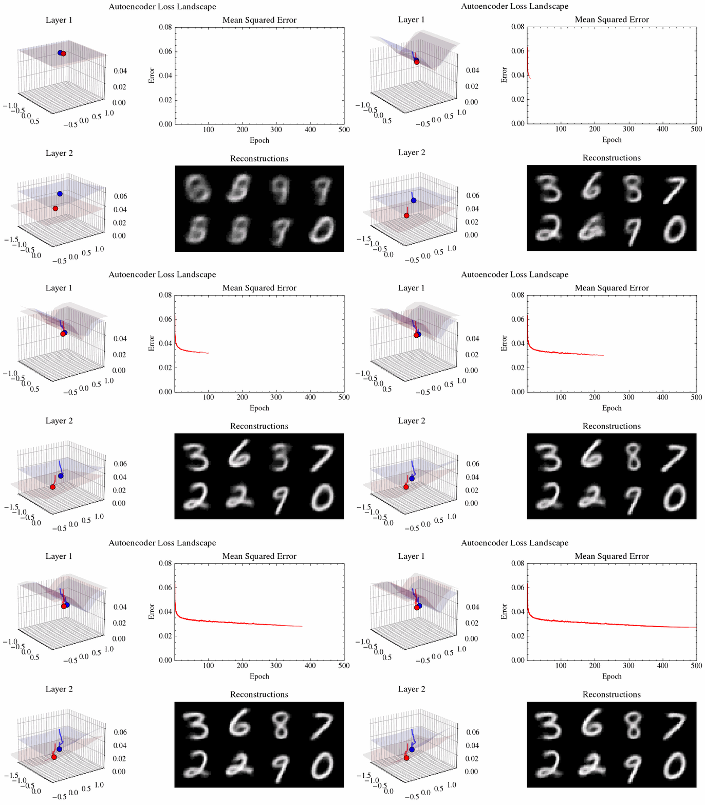
Reconstruction animation showing the Mean Squared Error curve, original digits, and reconstructions.

Image(filename=recon_filename)

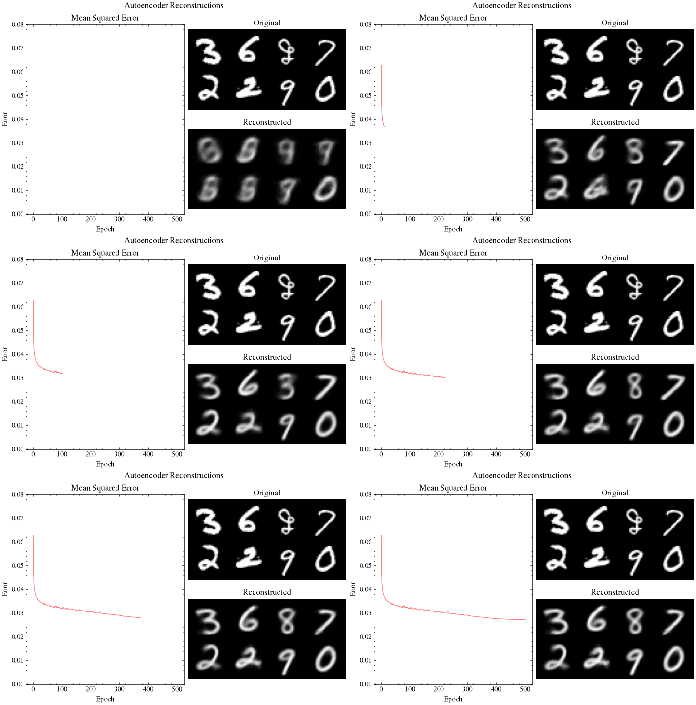
Latent Space Output GIF

Animation of the 2-neuron latent space. Each point is a validation image projected to \(z \in \mathbb{R}^2\) by the encoder, colored by its true digit. As training progresses, images of the same digit migrate together into distinct clusters — even though the autoencoder never sees the labels.

Image(filename=latent_filename)

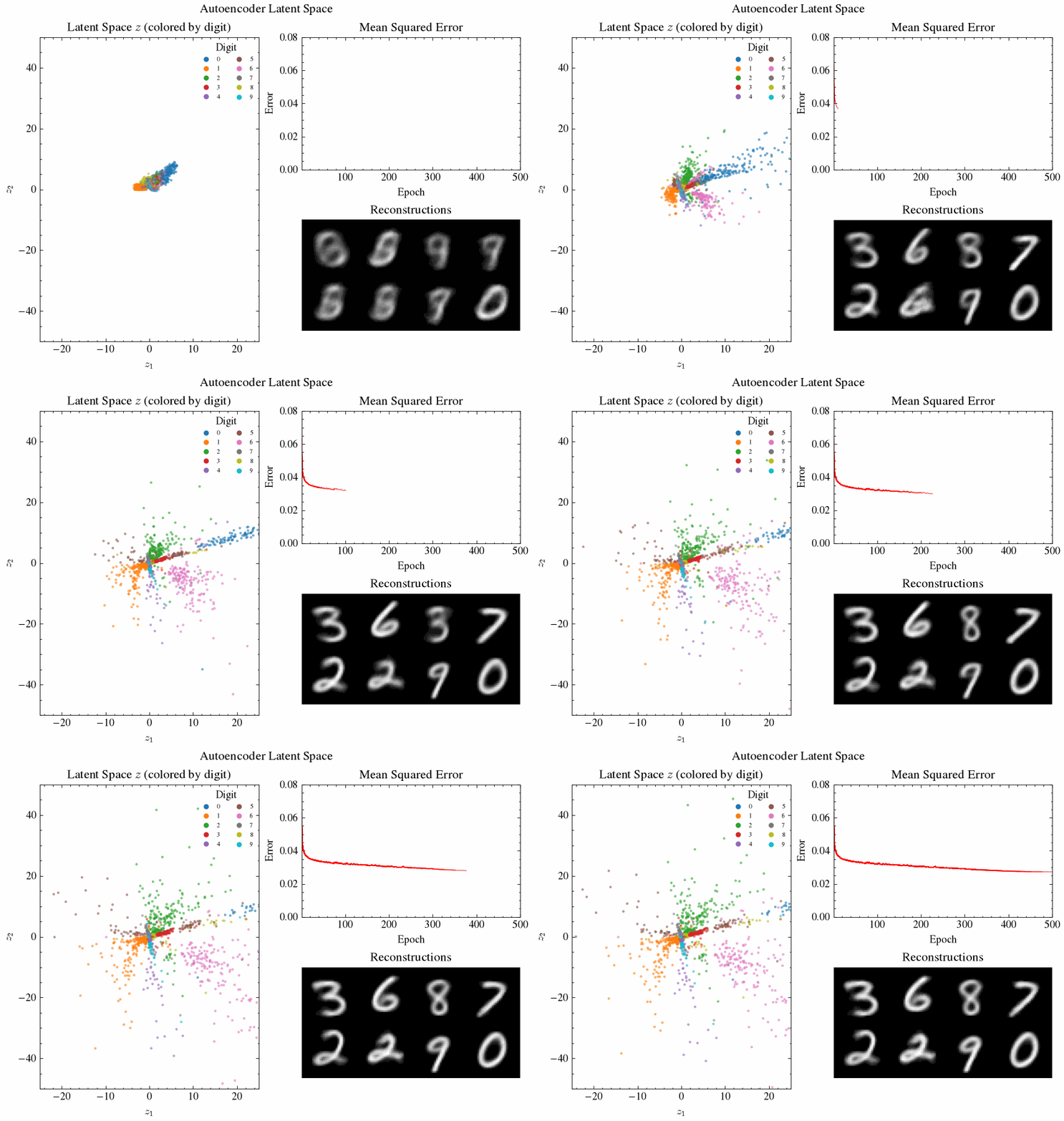
Loss Landscape Output GIF

Loss landscape animation with 3D surfaces for Layer 1 (encoder \(\text{Linear}(64, 2)\)) and Layer 2 (decoder \(\text{Linear}(2, 64)\)). The blue and red surfaces show how the MSE changes as two weights of each neuron are swept; the markers and trails trace the current weights descending through the landscape.

Set live_surface = True to recompute the surfaces every frame from the model’s current state (so the bowls deform as the rest of the network trains). This is slower — leave it False for a fast, fixed reference surface drawn once.

Image(filename=landscape_filename)