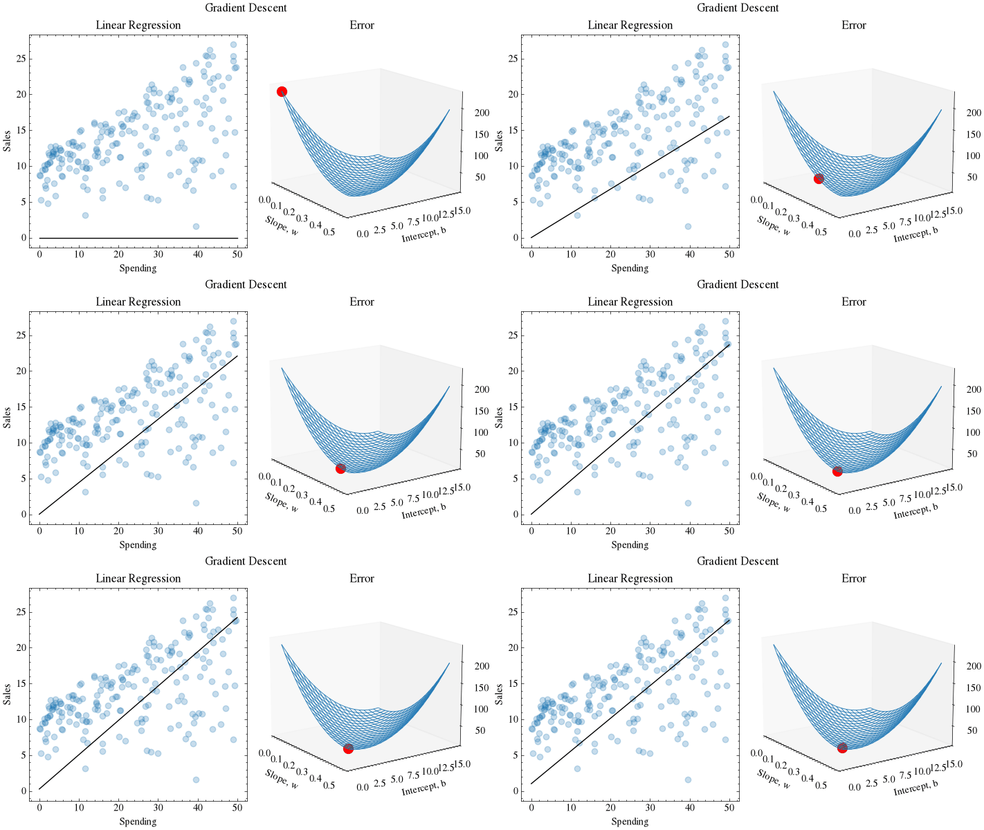
Gradient Descent

Gradient Descent is an algorithm that finds the local minimum of a function. This is applicable to machine learning because we want to find the optimal parameters that minimize our loss function. In machine learning, loss functions quantify the amount of error between the predicted values from a machine learning model and the actual expected values. In this notebook, we will perform linear regression by using gradient descent to find the optimal slope and y-intercept.

Training Dataset

Importing the libraries

import numpy as np
import matplotlib.pyplot as plt
import scienceplots
from IPython.display import display, Latex, Image
from celluloid import Camera

np.random.seed(0)
plt.style.use(["science", "no-latex"])

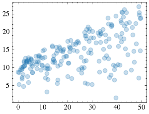
Let’s look at the training dataset. We will use columns 2 and 4 of the txt file. The linear regression model will find the optimal slope and y-intercept to fit the data.

fname = "REGRESSION-gradientDescent-data.txt"
x, y = np.loadtxt(fname, delimiter=",", unpack=True, skiprows=1, usecols=(2, 4))

fig = plt.figure()
ax = fig.add_subplot()
ax.scatter(x, y, color="#1f77b4", marker="o", alpha=0.25)

<matplotlib.collections.PathCollection at 0x7a9104ff5e20>

Loss Function: Mean Squared Error

For the linear regression model, the predicted value \(\hat{y}_i\) is the product of the weight \(w\) and the input feature \(x_i\) plus a bias term \(b\):

\[\hat{y}_i = w x_i + b\]

We will use the mean squared error function as our loss function:

\[\begin{split} \begin{align*} MSE &= \frac{1}{n} \sum_{i=1}^{n}(y_{i}-\hat{y}_i)^2 \\ &= \frac{1}{n} \sum_{i=1}^{n}(y_{i}-(w x_{i} + b))^2 \end{align*} \end{split}\]

Loss Function Gradient

def mse_loss(x, y, w, b):
    return np.mean(np.square(y - (w * x + b)))

In each epoch of gradient descent, a parameter is updated by subtracting the product of the gradient of the function and the learning rate (\(\eta\)). The learning rate controls how much the parameters should change. Small learning rates are precise, but are slow. Large learning rates are fast, but may overshoot and prevent the model from finding the minimum.

\[ \begin{align*} X_{t+1} = X_t - \eta \nabla f(X_t) \end{align*} \]

Since we are finding the optimal slope (\(w\)) and y-intercept (\(b\)) for our linear regression model, we must find the partial derivatives of the loss function with respect to \(w\) and \(b\).

Loss Function in Terms of W

Loss function with respect to \(w\):

\[\begin{split} \begin{align*} \frac{\partial}{\partial w} \left( MSE \right) &= \frac{\partial}{\partial w}\left[\frac{1}{n} \sum_{i=1}^{n}(y_{i}-(w x_{i} + b))^2\right] \\ &= \frac{1}{n} \sum_{i=1}^{n} \frac{\partial}{\partial w}\left[(y_{i}-(w x_{i} + b))^2\right] \\ &= \frac{2}{n} \sum_{i=1}^{n} (y_{i}-(w x_{i} + b))\frac{\partial}{\partial w}\left[y_{i}-(w x_{i} + b)\right] \\ &= \frac{2}{n} \sum_{i=1}^{n} (y_{i}-(w x_{i} + b))(-x_{i}) \\ &= -\frac{2}{n} \sum_{i=1}^{n} x_{i}(y_{i}-(w x_{i} + b)) \end{align*} \end{split}\]

def mse_loss_dw(x, y, w, b):
    return -2 * np.mean(x * (y - (w * x + b)))

Loss Function in Terms of b

Loss function with respect to \(b\):

\[\begin{split} \begin{align*} \frac{\partial}{\partial b} \left( MSE \right) &= \frac{\partial}{\partial b}\left[\frac{1}{n} \sum_{i=1}^{n}(y_{i}-(w x_{i} + b))^2\right] \\ &= \frac{1}{n} \sum_{i=1}^{n} \frac{\partial}{\partial b}\left[(y_{i}-(w x_{i} + b))^2\right] \\ &= \frac{2}{n} \sum_{i=1}^{n} (y_{i}-(w x_{i} + b))\frac{\partial}{\partial b}\left[y_{i}-(w x_{i} + b)\right] \\ &= \frac{2}{n} \sum_{i=1}^{n} (y_{i}-(w x_{i} + b))(-1) \\ &= -\frac{2}{n} \sum_{i=1}^{n} (y_{i}-(w x_{i} + b)) \end{align*} \end{split}\]

def mse_loss_db(x, y, w, b):
    return -2 * np.mean(y - (w * x + b))

Training the Linear Regression Model

Let’s define a function that uses the gradient algorithm to update the parameters of the loss function. The function uses the gradient functions we derived earlier.

General Gradient Descent Equation:

\[X_{t+1} = X_t - \eta \nabla f(X_t)\]

Weights Gradient Descent:

\[\begin{split} \begin{align*} w &= w - \eta \frac{\partial}{\partial w} [L(w, b)] \\ &= w - \eta \left[-\frac{2}{n} \sum_{i=1}^{n} x_{i}(y_{i}-(w x_{i} + b))\right] \end{align*} \end{split}\]

Bias Gradient Descent:

\[\begin{split} \begin{align*} b &= b - \eta \frac{\partial}{\partial b} [L(w, b)] \\ &= b - \eta \left[-\frac{2}{n} \sum_{i=1}^{n} (y_{i}-(w x_{i} + b))\right] \end{align*} \end{split}\]

def update_w_and_b(x, y, w, b, learning_rate):
    dw = mse_loss_dw(x, y, w, b)
    db = mse_loss_db(x, y, w, b)

    w = w - dw * learning_rate
    b = b - db * learning_rate

    return w, b

Graphing functions

Let’s define helper functions to plot the graphs.

def create_plots():
    plt.ioff()
    fig = plt.figure(figsize=(16 / 9.0 * 4, 4 * 1), layout="constrained")
    fig.suptitle("Gradient Descent")
    ax0 = fig.add_subplot(1, 2, 1)
    ax0.set_xlabel("Spending", fontweight="normal")
    ax0.set_ylabel("Sales", fontweight="normal")
    ax0.set_title("Linear Regression")

    ax1 = fig.add_subplot(1, 2, 2, projection="3d")
    ax1.set_xlabel("Slope, w")
    ax1.set_ylabel("Intercept, b")
    ax1.set_zlabel("Error")
    ax1.set_title("Error")
    ax1.view_init(15, -35)
    ax1.grid(False)

    camera = Camera(fig)
    return ax0, ax1, camera


def generate_error_range(x, y, N, w_max, b_max):
    w_vals = np.linspace(0, w_max, N)
    b_vals = np.linspace(0, b_max, N)
    w_range, b_range = np.meshgrid(w_vals, b_vals)

    error_range = np.zeros_like(w_range)
    for i in range(N):
        for j in range(N):
            error_range[i, j] = mse_loss(x, y, w_range[i, j], b_range[i, j])

    return w_range, b_range, error_range

Training the model

The train function will update the parameters in each epoch and update the visualization.

def train(x, y, w0, b0, learning_rate, epochs, output_filename):
    w = w0
    b = b0

    ax0, ax1, camera = create_plots()
    loss_dims = 20
    w_max = 0.5
    b_max = 15
    w_range, b_range, error_range = generate_error_range(
        x, y, loss_dims, w_max, b_max
    )

    X_plot = np.linspace(0, 50, 50)

    for e in range(epochs):
        # Capture and log at specific milestones and the final epoch
        if (
            (e == 0)
            or (e < 60 and e % 5 == 0)
            or (e % 1000 == 0)
            or (e == epochs - 1)
        ):
            # Redraw the loss landscape each frame so it appears in animation output.
            ax1.plot_wireframe(
                w_range, b_range, error_range, color="#1f77b4", linewidth=0.7, alpha=0.9
            )
            ax1.scatter([w], [b], [mse_loss(x, y, w, b)], color="red", s=100)

            # Plot regression data and current prediction line
            ax0.scatter(x, y, color="#1f77b4", marker="o", alpha=0.25)
            ax0.plot(X_plot, X_plot * w + b, color="black")

            # Log current training progress
            current_loss = mse_loss(x, y, w, b)
            print(f"epoch: {e:4d} | loss: {current_loss:.8f}")
            camera.snap()

        # Update parameters simultaneously
        w, b = update_w_and_b(x, y, w, b, learning_rate)

    animation = camera.animate()
    animation.save(output_filename, writer="pillow")
    plt.show()

    return w, b

Let’s train the linear regression model on a sample dataset.

fname = "REGRESSION-gradientDescent-data.txt"
x, y = np.loadtxt(fname, delimiter=",", unpack=True, skiprows=1, usecols=(2, 4))
output_filename = "gradient_descent.gif"
train(x, y, 0.0, 0, 0.00005, 4000, output_filename)

epoch:    0 | loss: 223.71625000
epoch:    5 | loss: 124.87289357
epoch:   10 | loss: 80.08948497
epoch:   15 | loss: 59.79711689
epoch:   20 | loss: 50.60004436
epoch:   25 | loss: 46.42952831
epoch:   30 | loss: 44.53621857
epoch:   35 | loss: 43.67456373
epoch:   40 | loss: 43.28028563
epoch:   45 | loss: 43.09774660
epoch:   50 | loss: 43.01113387
epoch:   55 | loss: 42.96798022
epoch: 1000 | loss: 41.62139410
epoch: 2000 | loss: 40.30390096
epoch: 3000 | loss: 39.06018012
epoch: 3999 | loss: 37.88724135

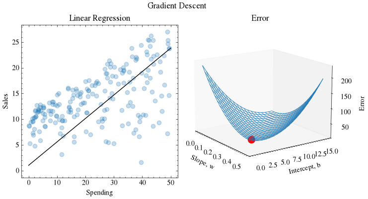
(np.float64(0.4560126699891239), np.float64(1.026884217380755))

Image(filename=output_filename)